Quick Answer: Probability distributions describe how data is expected to behave. Use our calculator to find probabilities, critical values, and visualize distributions like Normal, Exponential, Binomial, and Poisson — without manual tables or formulas.
Probability distributions are the foundation of statistics. They tell us how likely different outcomes are, from predicting exam scores to modeling website traffic. Whether you're running a hypothesis test, building a confidence interval, or analyzing risk, understanding distributions is essential.
Our Probability Distribution Calculator makes it easy to calculate probabilities, find critical values, and visualize distribution curves — all with real-time interactive charts.
1. What Are Probability Distributions?
A probability distribution is a mathematical function that describes the likelihood of different outcomes in a random process. Think of it as a blueprint for randomness.
Key concepts:
- PDF (Probability Density Function): Shows the relative likelihood of each value (for continuous distributions)
- PMF (Probability Mass Function): Shows the exact probability of each value (for discrete distributions)
- CDF (Cumulative Distribution Function): Shows the probability that a value is ≤ x
- Quantile (Inverse CDF): Finds the value x where P(X ≤ x) = p
Each distribution is defined by parameters (like mean μ and standard deviation σ for the Normal distribution) that control its shape and location.
2. The Normal Distribution: The Bell Curve
The Normal (Gaussian) distribution is the most important distribution in statistics. Its bell-shaped curve appears everywhere — from heights and IQ scores to measurement errors.
Parameters:
- μ (mu): Mean — the center of the distribution
- σ (sigma): Standard deviation — controls the spread
When to use: ✅ Measurement errors ✅ Natural phenomena (heights, weights) ✅ Averages of large samples (Central Limit Theorem) ✅ Z-tests and t-tests
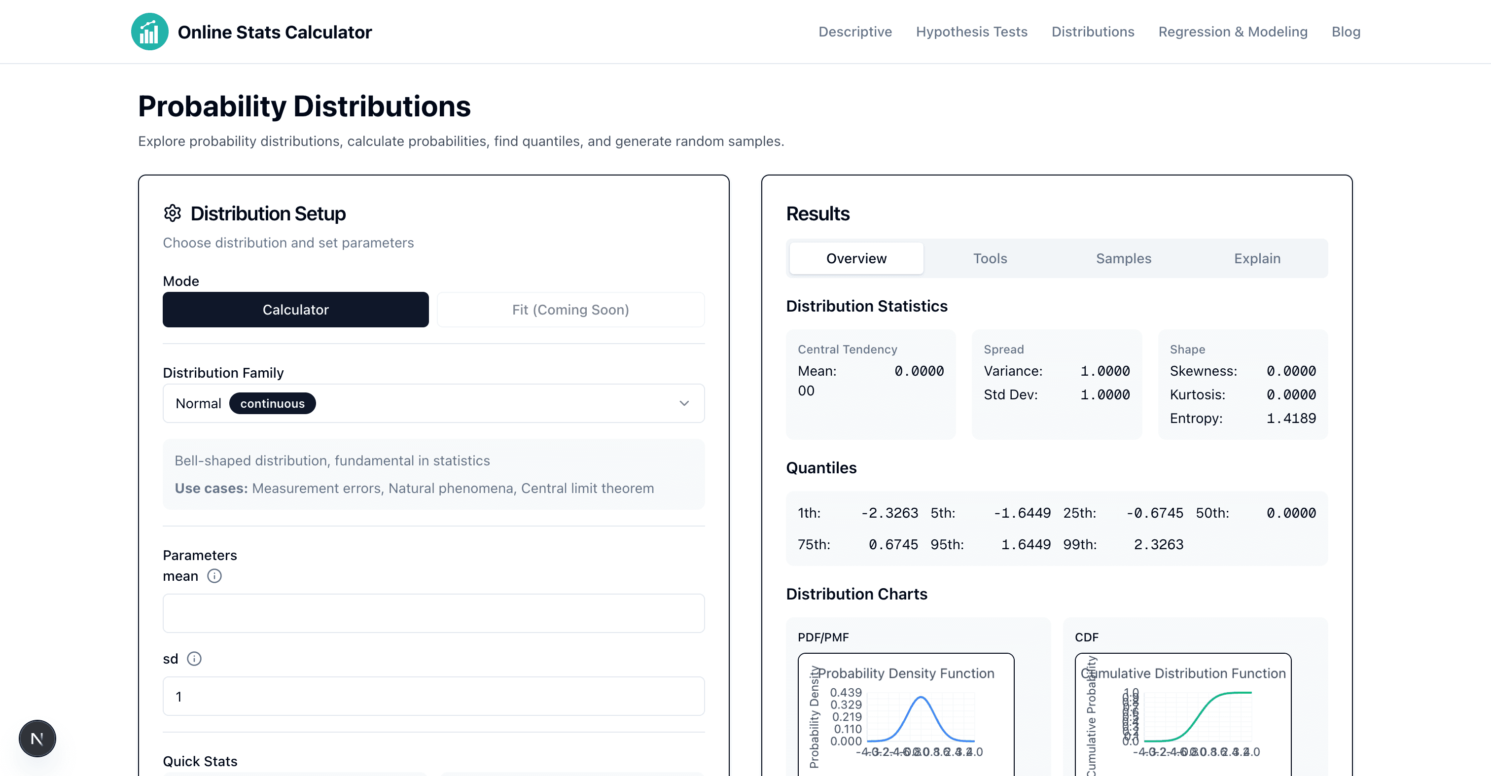
The Standard Normal Distribution (Z-distribution): When μ = 0 and σ = 1, we call it the standard normal distribution. This is used for z-scores and hypothesis testing.
Famous Result: For the standard normal distribution:
- P(X ≤ 1.96) ≈ 0.975 (97.5%)
- P(-1.96 ≤ X ≤ 1.96) ≈ 0.95 (95% confidence interval)
3. The Exponential Distribution: Time Between Events
The Exponential distribution models time until an event occurs in a Poisson process. It's memoryless — the probability of an event in the next hour is the same regardless of how long you've waited.
Parameters:
- λ (lambda): Rate parameter — average events per unit time
When to use: ✅ Time until equipment failure ✅ Customer arrival times ✅ Radioactive decay ✅ Time between earthquakes
Key properties:
- Mean = 1/λ
- Variance = 1/λ²
- Only one parameter needed
4. The Poisson Distribution: Counting Rare Events
The Poisson distribution counts discrete events occurring in a fixed interval of time or space. It's perfect for rare events.
Parameters:
- λ (lambda): Average number of events in the interval
When to use: ✅ Number of emails per hour ✅ Website visits per minute ✅ Defects per product ✅ Accidents per day
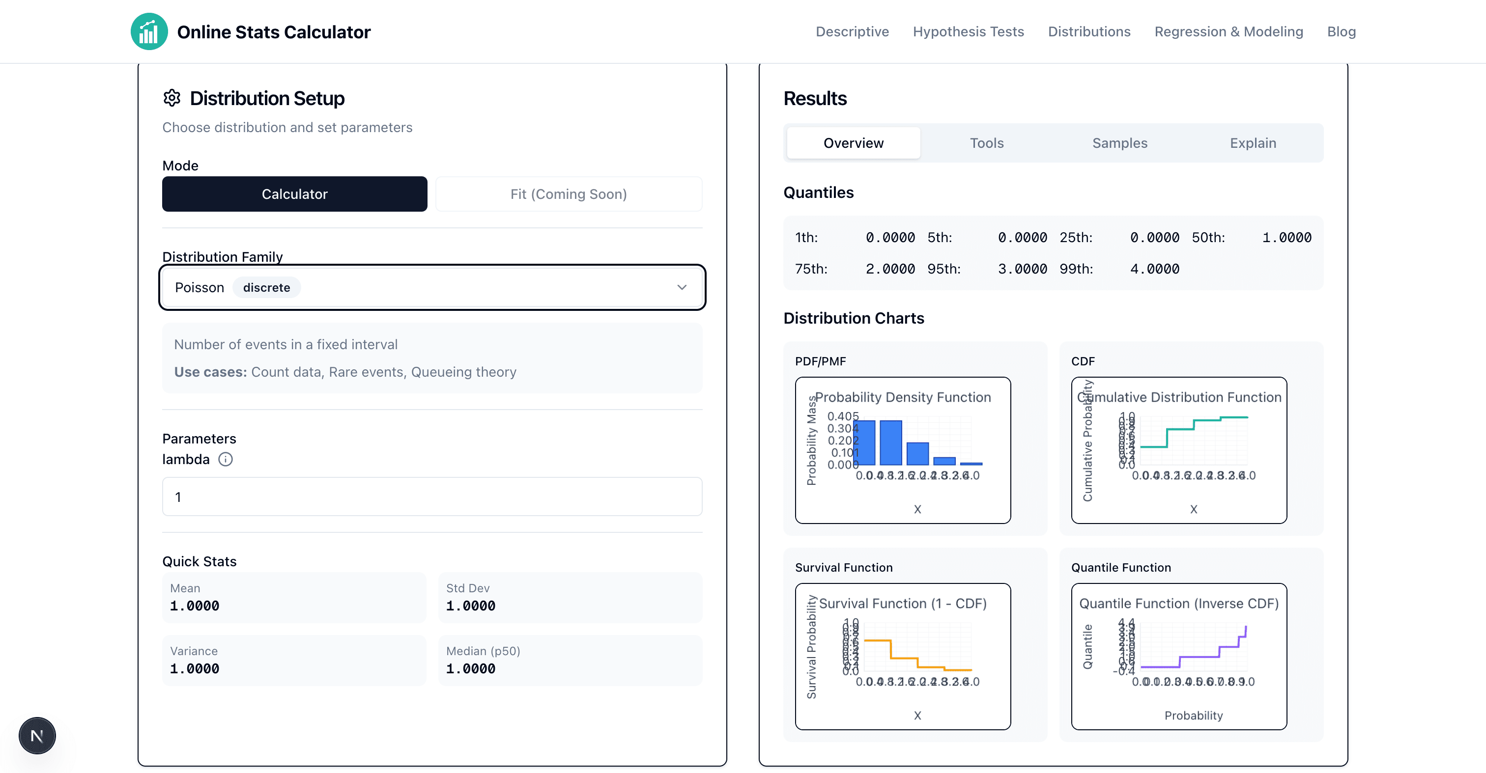
Key properties:
- Mean = λ
- Variance = λ (unique property!)
- Discrete values (0, 1, 2, 3, ...)
5. The Binomial Distribution: Success or Failure
The Binomial distribution models the number of successes in a fixed number of independent trials.
Parameters:
- n: Number of trials
- p: Probability of success on each trial
When to use: ✅ Coin flips (heads vs tails) ✅ Quality control (pass vs fail) ✅ Survey responses (yes vs no) ✅ Clinical trials (success vs failure)
Example: Flip a coin 20 times (n=20, p=0.5). What's the probability of getting exactly 12 heads?
The binomial distribution gives us: P(X = 12) ≈ 0.120
6. The Uniform Distribution: Equal Probability
The Uniform distribution assigns equal probability to all values in a range. It's the simplest continuous distribution.
Parameters:
- a: Minimum value
- b: Maximum value
When to use: ✅ Random number generation ✅ Modeling complete uncertainty ✅ Baseline for comparison
Key properties:
- Mean = (a + b) / 2
- Variance = (b - a)² / 12
- Flat PDF (constant height)
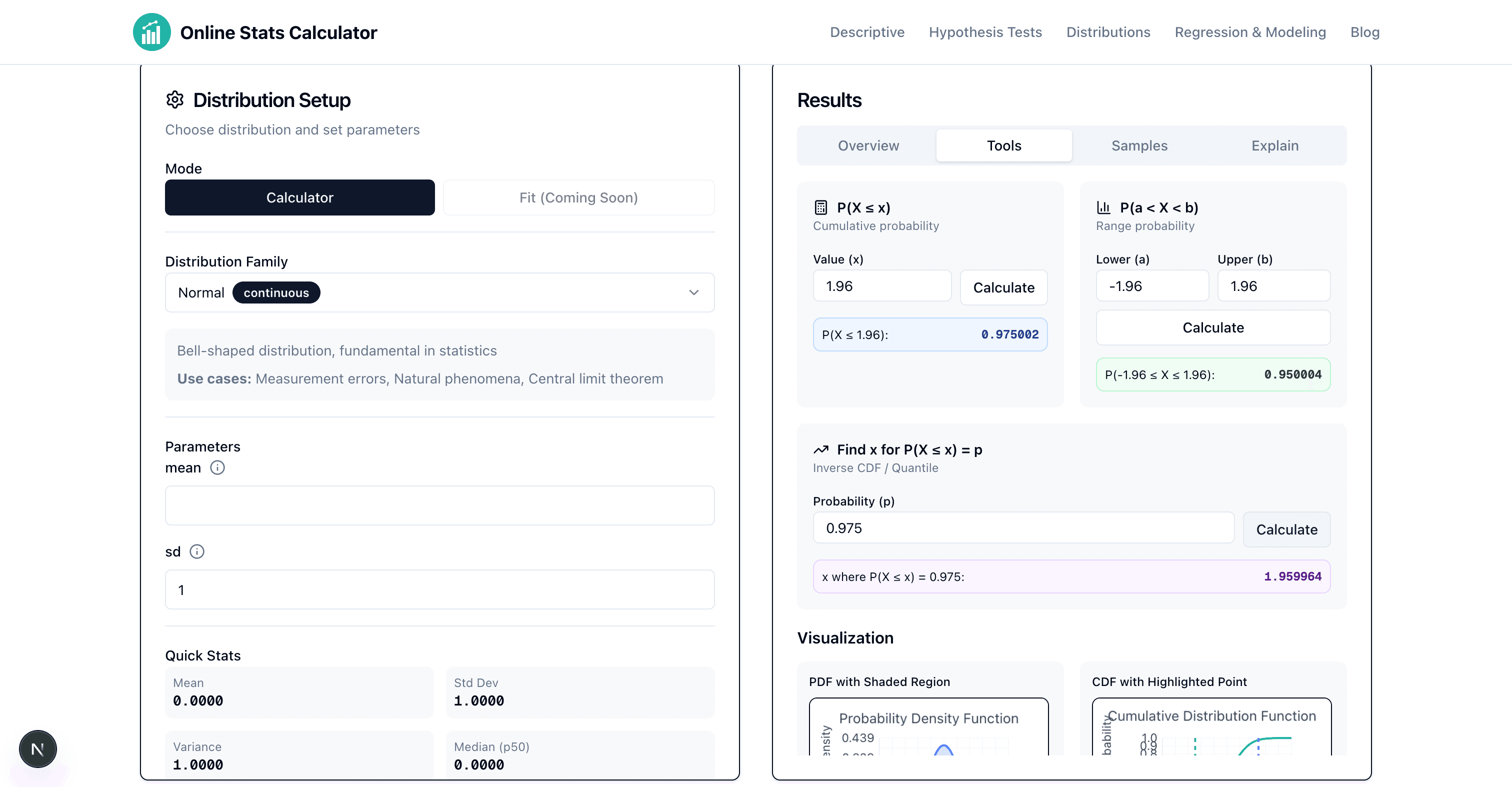
7. How to Use the Calculator
Let's walk through calculating probabilities step-by-step using our calculator.
Step 1: Choose Your Distribution
Navigate to the Distribution Calculator and select from the dropdown:
- Normal
- Exponential
- Uniform
- Poisson
Step 2: Set Parameters
Enter the required parameters for your chosen distribution. For example:
- Normal: μ = 0, σ = 1
- Exponential: λ = 1
- Poisson: λ = 5
- Binomial: n = 20, p = 0.6
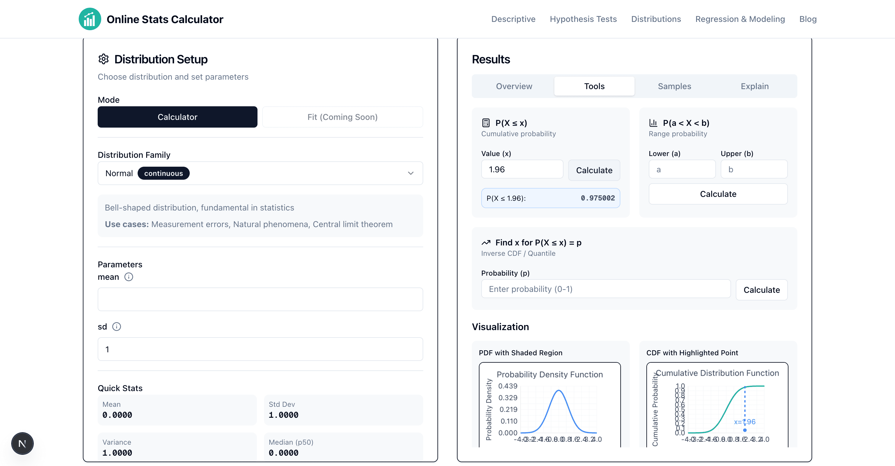
Step 3: Calculate Probabilities
Use the Tools tab for specific calculations:
P(X ≤ x) — Cumulative probability:
- "What's the probability a value is less than or equal to x?"
- Example: For Normal(0,1), P(X ≤ 1.96) = 0.975
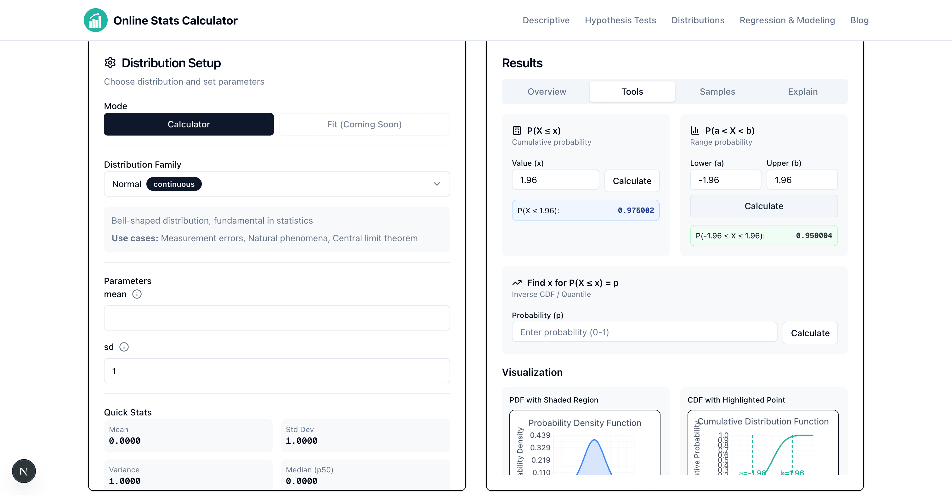
P(a < X < b) — Range probability:
- "What's the probability a value falls between a and b?"
- Example: P(-1.96 < X < 1.96) = 0.95 for standard normal
Find x for P(X ≤ x) = p — Inverse CDF (Quantile):
- "What value x has probability p below it?"
- Example: For p = 0.975, x = 1.96 (the 97.5th percentile)
8. Real-World Example: Quality Control
Scenario: A factory produces bolts with a target diameter of 10mm. Historical data shows diameters follow Normal(μ=10, σ=0.2).
Question 1: What percentage of bolts have diameter < 9.7mm?
Solution:
- Go to calculator, select Normal(μ=10, σ=0.2)
- Use P(X ≤ x) tool with x = 9.7
- Result: P(X ≤ 9.7) = 0.0668 → 6.68% are too small
Question 2: What diameter represents the 95th percentile?
Solution:
- Use Find x for P(X ≤ x) = p tool with p = 0.95
- Result: x = 10.329mm → 95% of bolts are smaller than 10.329mm
9. Understanding Critical Values
Critical values are specific points on a distribution used for hypothesis testing and confidence intervals.
Common critical values for Standard Normal (Z-distribution):
| Confidence Level | Two-Tailed | One-Tailed |
|---|---|---|
| 90% | ±1.645 | 1.282 |
| 95% | ±1.960 | 1.645 |
| 99% | ±2.576 | 2.326 |
How to find them:
- For 95% two-tailed: α = 0.05, α/2 = 0.025
- Upper critical value: P(X ≤ z) = 1 - 0.025 = 0.975
- Use inverse CDF: z = 1.96
💡 Tip: For small samples (n < 30), use the t-distribution instead of Normal. The t-distribution has heavier tails to account for additional uncertainty.
10. Distribution Selection Guide
| Distribution | Type | When to Use | Example |
|---|---|---|---|
| Normal | Continuous | Symmetric data, averages, natural phenomena | Heights, test scores, errors |
| Exponential | Continuous | Time between events (memoryless) | Equipment failures, arrivals |
| Uniform | Continuous | Equal probability across range | Random number generation |
| Binomial | Discrete | Count successes in fixed trials | Coin flips, quality control |
| Poisson | Discrete | Count rare events in interval | Emails per hour, defects |
11. Common Use Cases & Best Practices
Hypothesis Testing
Probability distributions power statistical tests:
Z-test (Normal): Compare sample mean to population when σ is known t-test: Compare means when σ is unknown (use t-distribution) Chi-square test: Test independence or goodness-of-fit Binomial test: Test proportions in small samples
Confidence Intervals
Build confidence intervals using quantiles:
95% CI for mean: x̄ ± 1.96 × (σ/√n) for large samples 95% CI for proportion: Use Wilson score interval (more accurate)
Quality Control
Set control limits using the Normal distribution:
- Upper Control Limit (UCL): μ + 3σ (captures 99.7%)
- Lower Control Limit (LCL): μ - 3σ
Risk Analysis
Model uncertainty in business decisions:
- Financial returns: Often approximately Normal
- Insurance claims: Use Exponential or Gamma
- Project completion: Use Beta or triangular distributions
Pro Tip: Always check your distribution assumptions! Use:
- Q-Q plots to visually assess normality
- Shapiro-Wilk test for formal normality testing
- Histogram + density plot to visualize your data's shape
12. Summary & Quick Reference
Key Takeaways:
- Normal distribution is your go-to for symmetric, bell-shaped data
- Exponential models time between events (memoryless)
- Poisson counts rare events in fixed intervals
- Binomial counts successes in fixed trials
- Use P(X ≤ x) for cumulative probability
- Use inverse CDF to find critical values and percentiles
Calculator Workflow:
- Select distribution type → 2. Set parameters → 3. Choose calculation type → 4. Interpret results
👉 Ready to practice? Try the Probability Distribution Calculator now with the examples from this guide!
Download Practice Data:
- Distribution Examples CSV — sample data for each distribution type
Need help with other statistical analyses?
- Descriptive Statistics Calculator — Mean, median, mode, standard deviation
- Confidence Intervals Calculator — Build confidence intervals for means and proportions
- Hypothesis Testing Calculator — Perform t-tests, z-tests, and more